Machine Learning of Multiphase Flows
I built and developed machine learning frameworks for predicting flows in engineering devices. My study was the first of its kind that can predict spatiotemporally varying and statistically stationary flows.
Spatiotemporally Varying Flows
Flows varying in both space and time, such as transient flows and unsteady flows.
Machine Learning Framework
The framework was developed in four steps. The Machine Learning (ML) algorithm of choice were Gaussian Processes with the capability to build complex kernel functions to emulate canonical flow configurations. Reduced Order Modeling (ROM) was conducted on spatiotemporally varying flows to reduce dimensionality of the flow.
Predicting Flow Modes
ROM was achieved through Proper Orthogonal Decomposition (POD) and predictions were made for the corresponding mode number for the testing points. For the canonical configuration of flow over a cylinder, 16 modes are needed to capture 99% of the flow. Galerkin reconstruction was utilized to reconstruct the spatio-temporal flow.
Flow over a Bluff Body
The timesteps for the testing condition of Reynolds Number (Re) of 185 are reconstructed with the predicted spatial modes and time coefficient vectors. The flowfield is reconstructed using Galerkin reconstruction and the results are compared actual simulation for error quantification, using L1 norm.
Jet Injection into Quiescent Chamber
Timesteps for the testing condition of injection velocity of 22.5 m/s are reconstructed using Galerkin reconstruction and the the results compared with a simulation for error quantification, using the L1 norm.
Stationary Flows
Flows that do vary in space but not in time, such as statistically stationary and steady-state flows.
Machine Learning Framework for Stationary Flows
This framework involves three steps for machine predicting the flowfield for a liquid jet injected into heated crossflowing air. The Machine Learning (ML) algorithm of choice were Gaussian Processes. Dimensionality reduction was not needed as this involves only spatial data for the flowfield. Temporally the flow does not vary - i.e. statistically stationary or steady flow.
Turbulent Kinetic Energy
Turbulent kinetic energy (TKE) comparison for momentum flux ratios (q) of 7 and 40 with real data from simulations. The L1 error is - ~10.47% for q = 7; ~13.25% for q = 40.
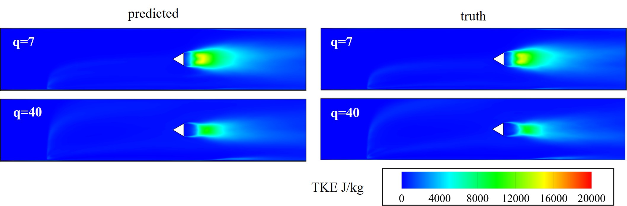
TKE contours for q=7 and q=40.
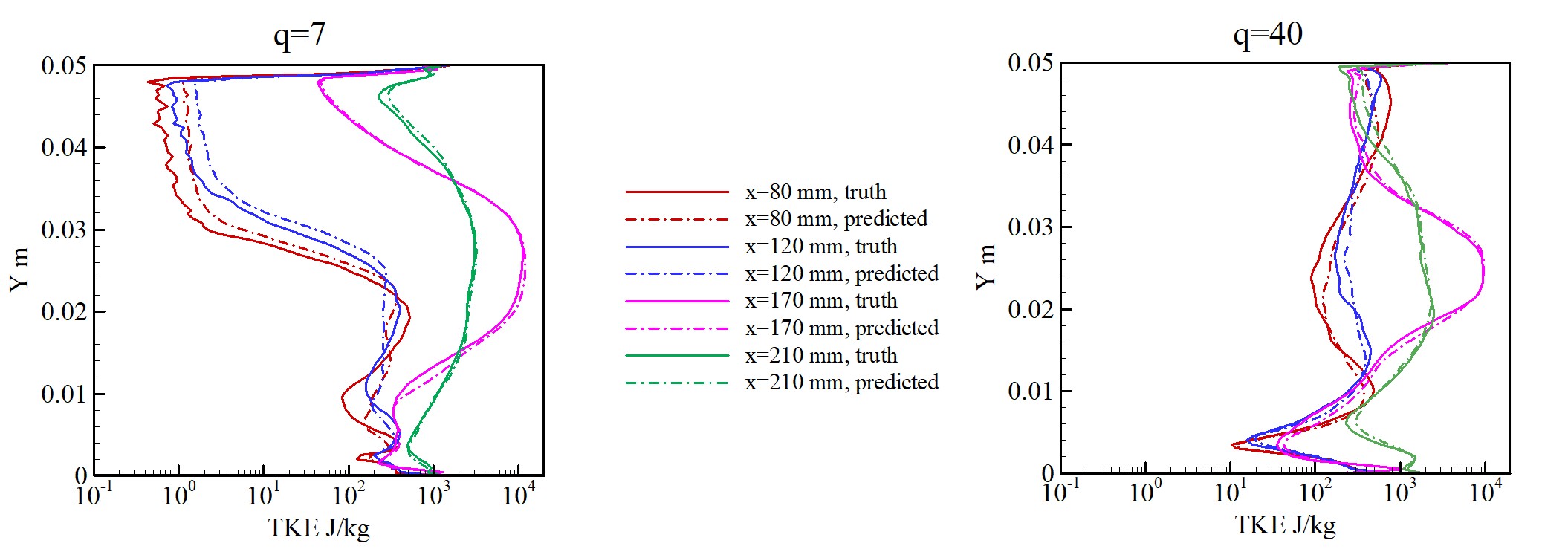
Comparison of TKE along the height at different locations from the left edge for q=7 and q=40.
Vapor Fraction of a Liquid Jet Injection
Vapor fraction comparison for momentum flux ratios of 7 and 40 with real data from simulations. The L1 error is - ~11.91% for q = 7; ~7.99% for q = 40.
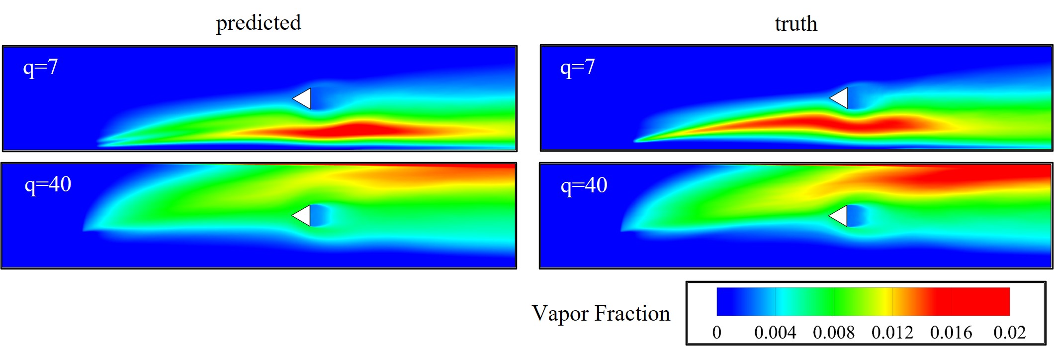
Vapor fraction contours for q=7 and q=40.
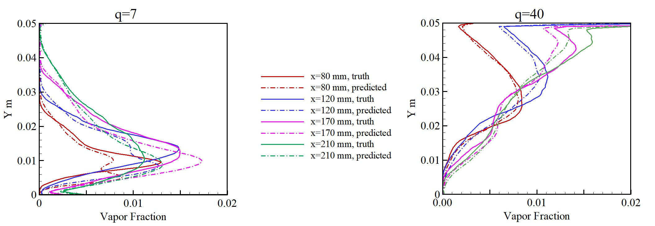
Comparison of vapor fraction along the height at different locations from the left edge for q=7 and q=40.
Performance Comparison of Machine Learning Algorithms
As different machine learning algorithms are developed, one has to have a good understanding of their performance to select the most suitable algorithm for accuracy and training speedup purposes. To demonstrate this, I modified Gaussian Processes to work with multiple independent variables and compared its training and prediction accuracy with a deep neural network.
Change in Contour Resolution with Number of Training Points
Changing the number of training points alters the training surface significantly making it very feature rich. This change necessitates the altering of kernel functions or the neural network architecture to achieve better results for accuracy and speedup.
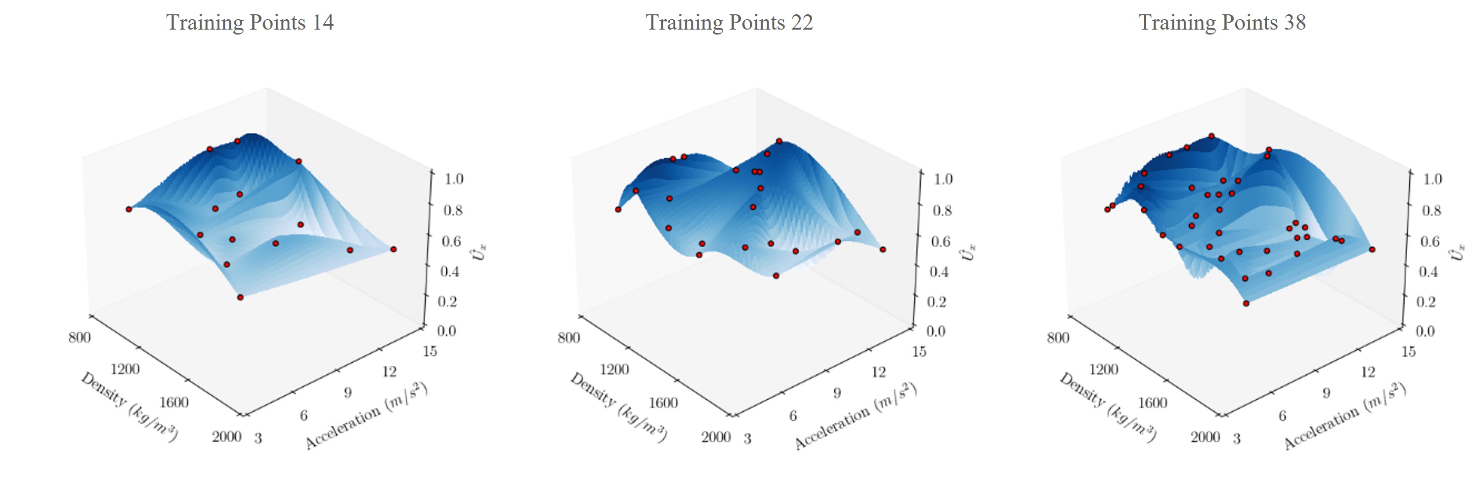
Training surface contours for velocity component with two independent variables - density of lighter fluid and acceleration for a Rayleigh-Taylor instability.
Comparison of Machine Learning Predictions for the Rayleigh-Taylor Phenomenon
Comparison of Gaussian Process (GP) and Neural Network (NN) based surrogate models for accuracy with actual simulation data or truth for a Rayleigh-Taylor instability.
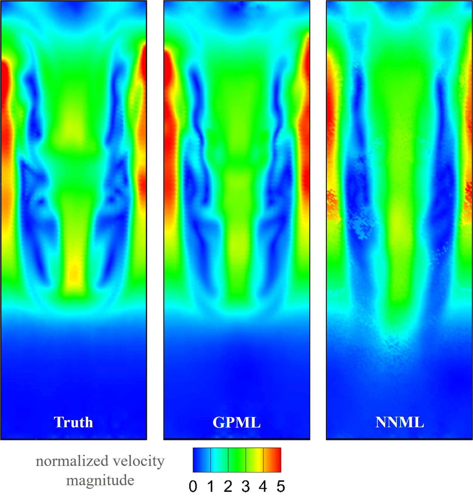
L1 errors - GP ~ 20%; NN ~34%. Training times - GP ~1.5 hours; NN ~126 hours.
Machine Learning & High-Speed Flows
More updates coming soon.
Relevant Publications
- Ganti H, “Data-Driven Surrogate Modeling of Two-Phase Flows”, PhD Thesis, April 2023. http://rave.ohiolink.edu/etdc/view?acc_num=ucin1684772398259224.
- H. Ganti, M. Kamin, P. Khare, "Design Space Exploration of Turbulent Multiphase Flows Using Machine Learning-Based Surrogate Model" Energies, September, 2020. doi: https://doi.org/10.3390/en13174565.
- H. Ganti, P. Khare, “Data-Driven Surrogate Modeling of Multiphase Flows Using Machine Learning Techniques”, Computers and Fluids, October 2020. doi: https://doi.org/10.1016/j.compfluid.2020.104626.
- Ganti H, Kamin M, Khare P., “Design Space Exploration for Liquid Jet Vaporization in Air Crossflow using Machine Learning”. AIAA SciTech Forum & Exposition, January, 2019. doi: https://doi.org/10.2514/6.2019-2211.
- Ganti H, Khare P., “Prediction of Liquid Jet Atomization Using Gaussian Process Based Machine Learning Techniques”. 14th Triennial International Conference on Liquid Atomization and Spray Systems, July, 2018.
- Ganti H, Khare P., “Spatio-Temporal Prediction of Gaseous and Liquid Spray Fields using Machine Learning”. July, 2018 Joint Propulsion Conference, AIAA. doi: https://doi.org/10.2514/6.2018-4760.